Knowledge Base

Welcome! The articles below are meant to help you answer your questions about our technology. If you have more questions please direct them to info@orylphotonics.com

Dissecting the Membrane Association Mechanism of Aerolysin Pores at Femtomolar Concentrations Using Water as a Probe

In this scientific article published in Nano Letters, Second Harmonic Scattering is used to probe the membrane association mechanism of aerolysin pores.

Here the researchers measures changes in the SHS of water completely in solution, without any requirement of coupling to a surface. SHS is indeed really a label-free sensing technique (no tags, fluorophores or even protein absorbance). See the full paper here.

Are you struggling to profile the solubility and aggregation of your precious APIs?

A drug must be absorbed by the body to reach its intended biological target. However, before reaching its destination, and depending on the type of delivery, a drug will be exposed to various environments [1]. For an oral delivery, the drug experiences various pH and media conditions (from enzymes to bile salts, etc), going from the mouth (pH 6.5–7.5) to stomach (pH 1.5–3.5) to small intestine (gradual pH increase from 5.5 to 8) and large intestine (6.0–7.0).

Therefore, the solubility and aggregation of drug molecules depends on multiple experimental parameters (temperature, ionic strength, salts, presence of excipients, etc) as well as on the different types of solvents and media conditions. From a formulation point-of-view, all these aspects should be considered to make sure that the drug remains potent and bioavailable [2].

The challenges with profiling

However, profiling solubility and aggregation is a challenging endeavour, for several reasons.

1. Profiling is resource intensive

  • It requires excess drug substance, which is problematic for expensive or scarce APIs
  • It requires skilled labor with extensive hands-on work
  • It requires expensive and complex instrumentation

The cost of producing new drugs has steadily increased in the past years [3]. Especially with new drug modalities, such as biologics, gene therapies, and cell therapies which are generally more expensive to develop [4]. Moreover, the analytical development for these types of drugs is at an early stage. New tools and method developments are needed to address the solubility and aggregation profile of new drug modalities with particular focus on miniaturization, universality and flexibility (studying drugs in their native environment), and sensitivity.

2. Profiling is slow, uncertain and risky

  • It is necessary before project initiation
  • Current technologies are slow and stifle the development

Ideally, before any drug development occurs, the solubility and aggregation landscape should have been profiled. However, this challenge is overwhelming because of the enormous the amount of material needed to profile the solubility and aggregation landscape of a drug. A technology is needed that requires the least amount of compound – especially for expensive drugs where it is almost impossible to perform any type of solubility/aggregation profiling.

3. Profiling is constraint by production:

  • There is pressure to develop, but many potential formulations pathways to choose
  • Aggregation curbs manufacturing

Indeed, once the drug enters the drug product phase, there is a pressure to increase its production. However, if the aggregation profile is not yet optimized, the yield will be low and process improvements must be a top priority. To optimize the process, aggregation profiling is a must and should be obtained with speed and precision.

These difficulties are important; hence scientists and technicians are left with little coping strategies. Either by measuring only a few conditions assumed to be key, or by delaying the study only when problems happen. In a nutshell: you have to make tough choices by sacrificing either knowledge or resources.

Rethinking solubility and aggregation profiling: Oryl’s solution

Oryl has developed a groundbreaking technology to measure drug aggregation and solubility using a patented ultrafast laser-based second harmonic scattering (SHS) method. This optical phenomenon measures how the solvent redistributes around the solute molecules (what we call the Solvent Redistribution method) to follow the dynamics of solubility and aggregation in an accurate, fast and resource-saving way. The key advantage of this method is its minimal sample requirement, using only 10 µg per solubility datapoint.

Unlike HPLC-based systems that require over 1 mg of compounds, Oryl’s method allows you to obtain around 100 solubility datapoints from the same amount. This enables large-scale solubility and aggregation profiling. Additionally, since the technology uses light-scattering and standard well-plates without destroying the sample, you can perform time-lapse and dynamic measurements and reuse the sample for other complementary techniques.

In a nutshell, Oryl’s method allows rapid, accurate and actionable feedback to orient the drug development using as little compound as possible. This versatile technology works with both small and large molecules in any dipolar solvent, allowing you to profile conditions across various salt concentrations, excipients, and solvents.

References

[1] Advances in Oral Drug Delivery for Regional Targeting in the Gastrointestinal Tract – Influence of Physiological, Pathophysiological and Pharmaceutical Factors
[2] Advances in Oral Drug Delivery Systems: Challenges and Opportunities
[3] Costs of Drug Development and Research and Development Intensity in the US, 2000-2018
[4] Small molecules vs. Biologics: Understanding the differences

Benchmarking the Solvent Redistribution method

We performed solubility measurement of several poorly soluble compounds following the protocol described in figure 1. A standard 384 well-plate (Greiner 384 Well UV Star, ref. 781801) is used and the plate layout is described in figure 2. Using an acoustic liquid dispenser robot (Echo Labcyte), an increasing concentration (0, 0.1, 1, 2.5, 5, 7.5, 10, 25, 50, 75, 100 µM ) of the test compound is transferred across the 384 well-plate (dilution by row). After adding the compounds, a peristaltic liquid dispenser robot is used to transfer 100 µL of PBS buffer to each well-plate. The 384 well-plate is then directly tested in Oryl’s instruments after a 2-hour incubation period. There are 20 compounds that were tested with N=5 replicates. For comparison, the same set of compounds are tested with nephelometry. For some of the compounds, the solubility limit was measured using HPLC-UV method, with centrifugation as a pre-step to remove big aggregates and injecting the supernatant to HPLC-UV for determining the concentration of the dissolved compounds. The results are shown in Table 1.

1. Direct transfer of stock solution

2. Addition of solvent

3. Direct screening and analysis

Figure 1: Protocol for fully automated solubility measurement process. The full process of solubility measurement can be automated with liquid handling robots and the Solvent Redistribution method. In step 1, an acoustic liquid dispenser (Labcyte, Echo platform) is used to directly transfer the stock solution into well-plates with increasing concentration. In step 2, the solvent is added with peristaltic liquid dispenser (100 µL of volume). Lastly, the well-plate is measured with Oryl’s instrument. The analysis is performed automatically with Oryl’s software.

Figure 2: Experimental well-plate layout. Greiner 384 Well UV Star is used in the benchmarking study. The total volume per well is 100 µL. The solvent is PBS buffer with pH 7.4. There are 5 replicates per compound and the compound concentration is increased along each row with concentration range: 0, 0.1, 1, 2.5, 5, 7.5, 10, 25, 50, 75, 100 µM.

Table 1: Benchmarking the Solvent Redistribution method with nephelometry and HPLC-based solubility measurements. The values for Solvent Redistribution and nephelometry are measured kinetic solubility limit (in micromolar – µM) for the 20 compounds. For HPLC-based measurements, some are done in-house while the rest are taken from literature values (see superscript for reference).

CpdReplicate 1Replicate 2Replicate 3Replicate 4Replicate 5Average OrylHPLC-UVNephelometry
15.615.614.834.934.415.0813.1#90.73
28.046.797.733.696.856.624^51.78
33.343.053.273.053.763.299^29.4
499.9799.9799.9799.9799.9799.97*->100
50.020.030.030.020.020.024.36**26.87
621.2228.3628.0726.1825.1525.793^26.55
70.200.350.331.100.840.567.538.4
87.656.797.505.565.906.687^38.3
999.9799.9797.9999.9799.9799.57*->100
106.145.565.615.455.235.600.110.7
111.485.721.946.527.504.63121.2
127.811.283.085.346.794.86112.8
135.285.033.924.503.844.512.5^7.71
1499.9799.9799.9799.9799.9799.97*-> 100
1516.527.428.985.235.568.7412.7#22.40
160.700.100.260.261.160.50-7.85
177.816.526.657.815.726.902^51.02
1815.1017.2013.5316.3619.5916.36121.7
191.501.793.442.682.872.4619.1#7.11
200.010.140.092.350.010.520.117.5
* compound is soluble
# Advanced Drug Delivery Reviews 59 (2007) 546-567, pH 6.5 in 50 mM phosphate buffer
^ Anal. Chem. 2009, 81, 3165–3172, pH 7.4, HEPES buffer
** Assay Drug Dev. Technol. 2007, vol 5, no. 4

Figure 3: Summary of the measured solubility values for 20 compounds by directly comparing the Solvent Redistribution method, nephelometry and HPLC-UV based measurements.

Figure 3 shows that the Solvent Redistribution method is comparable in terms of sensitivity to HPLC-UV method, with both methods more sensitive than nephelometry. In table 3, some of the values for HPLC-UV are obtained from literature (see superscript). It should be noted that these values should be taken carefully as there is a huge spread in the variability of solubility values in literature (see Perspectives in solubility measurement and interpretation doi: 10.5599/admet.686).

Results

Table 1 and figure 3 clearly shows that The Solvent Redistribution method produces sensitive and reproducible measurements. Although 5 replicates were used in this study, the results show reproducible measurements that 3 replicates are more than sufficient. Figures 4-6 show some selected solubility plots that demonstrate its sensitivity and accuracy. The key feature of the Solvent Redistribution method is the repeatable baseline measurements with std/mean < 5%. With this precision, it is straightforward to detect the jump in intensity that corresponds to the solubility limit and allows for automated solubility analysis. We define a threshold as mean + 3*standard deviation of the baseline, with the baseline defined as average intensity of the 2 lowest concentrations. The solubility limit is calculated as the concentration at which the threshold is reached (see figure 4).

Figure 4: Solubility analysis plot for Compound 18. Right plot: full concentration range. Left plot zooms in the concentration range 1-10 µM showing the jump in intensity.

Figure 5: Solubility analysis plot for Compound 1. Right plot: full concentration range. Left plot zooms in the concentration range 1-10 µM showing the jump in intensity.

Figure 6: Solubility analysis plot for Compound 16.Right plot: full concentration range. Left plot zooms in the concentration range 1-10 µM showing the jump in intensity.

Conclusion

The Solvent Redistribution method is able to detect the solubility limit of drug-like compounds (mostly small molecules) providing results that are comparable to HPLC-UV and more sensitive than nephelometry. The full solubility measurement process is automated: from sample preparation using acoustic robot and peristaltic liquid dispenser to direct screening and analysis with Oryl’s instrument. The Solvent Redistribution method provides high-throughput and reproducible measurements with excellent sensitivity (<1 µM, small molecules). Combined with minimum use of compounds, the Solvent Redistribution method opens-up new avenues to perform solubility measurements at scale. Example applications are characterization of compound libraries, hit validation in early state drug discovery to solubility debugging with different solvents, pH and excipient combinations.

Acknowledgements

All the experiments presented in this benchmarking was done in collaboration with the Biomolecular Screening Facility (BSF) at EPFL. We express our gratitude to the BSF team, specifically Antoine Gibelin, Jonathan Vesin, Marc Chambon and Prof. Gerardo Turcatti.

Rapid and sensitive solubility measurement with minimum quantity of compounds

If we are to create a wish list for solubility measurement, what would it be? The ideal solubility measurement should be rapid, sensitive  and using minimum amount of compounds. It must have a wide application coverage (different samples, solvents, pH, temperatures, excipients) and should deliver reproducible results. Preferably, the full process from sample preparation to measurement and analysis is fully automated to minimize errors and decrease hands-on time.

Is this possible? It is now. How? Using The Solvent Redistribution Method from Oryl Photonics.

Solubility measurement with the Solvent Redistribution method

Minimal quantity

~2 μL of stock solution per solubility datapoint

Sensitive and accurate

< 1 μM small molecules,  low error std/mean < 5%

Rapid and high-throughput

1-100 ms read time per well, automated process

The Solvent Redistribution (SR) method detects the solubility and aggregation of compounds by measuring how the solvent redistributes around the solute molecules as they transition from monomeric state to aggregated state (dimers, trimers, etc) as shown in Figure 1. The SR method detects the onset of aggregation at concentrations below the range where turbidity occurs. It is thus more sensitive than turbidity measurements while retaining the advantage of speed. Additionally, it is precise with exceptional reproducibility. Visit this page for a detailed benchmarking study.

Figure 1: Schematic of aggregation for the Solvent Redistribution method. With increasing solute concentration, solute monomers transition to stable aggregates. In-between fully dissolved monomers and stable aggregates, there is a concentration range where different types of structures (dimers, trimers, etc.) co-exist. The distribution of solvent molecules around these structures change dynamically – hence the term Solvent Redistribution. Relative to the monomer state, there is an increase in the number of solvent molecules around the solute at the onset of aggregation that can be used a metric to detect the solubility limit.

Figure 1 shows the figure of concept for the SR method. With increasing concentration, the solute transitions from monomers to stable aggregates. Within the transition phase, there exists a dynamic phase of different types of structures (dimers, trimer, quadrimers, etc.) that is characterized by a higher degree of structural anisotropy. Correspondingly, the solvent around these structures redistributes and fluctuates, hence the term Solvent Redistribution. The Solvent Redistribution method is based on high-efficiency second harmonic (SH) scattering that directly measure the interfacial solvent redistributions. At the onset of aggregation (nucleation), there is an increase in the number of interfacial solvent molecules that leads to a steep increase in the SH intensity – this is used as a metric to measure the solubility limit.

Unique sensitivity

The SR method is uniquely sensitive because of:

  1. Wavelength separation between incoming and second harmonic beams – second harmonic photons are emitted at twice the frequency of the incoming beam (515 nm emitted, 1030 nm incoming beam) providing background-free measurements;
  2. Second harmonic scattering originates from the anisotropic distribution of the solvent which provides structural sensitivity and makes it selective to how substances aggregate;
  3. Pulsed laser that allows to synchronize the second harmonic signal with the detector.

These factors improve the signal-to-noise ratio of the SR method providing exceptionally reproducible measurements.

Minimum quantity of compounds

Since it is based on light scattering, the SR method requires minimum amount of compound and chemicals. With standard 384 well plates (or 96 half-area well plates) using 100 µL of volume, the compound requirement is typically around 2 µL of 10 mM stock solution per solubility datapoint (target maximum concentration of 100 µM). With N=3 replicates, it is now feasible to obtain solubility data per compound with ~6 µL of compound. Table 1 details the compound requirement depending on the target screen concentration (for example, if we want to qualify compounds to be soluble within a defined range of target screen concentration).

Table 1: Compound consumption with the SR Method. The compound requirement per solubility datapoint is ~4× of the target screen concentration.

Target Screen (µM)Volume required per solubility datapoint (µL)Total volume required (µL) for N=3 replicates
100.41.2
200.82.4
501.03.0

Automated and high-throughput solubility measurement

Direct transfer of stock solution

Addition of solvent

Direct screening and analysis

Figure 2: Fully automated solubility measurement process. The full process of solubility measurement is automated with liquid handling robots and Oryl’s SR method. In step 1, an acoustic liquid dispenser (Labcyte, Echo platform) is used to directly transfer the stock solution into well-plates with increasing concentration. In step 2, the solvent is added with peristaltic liquid dispenser (50 or 100 µL of volume). Lastly, the well-plate is measured with Oryl’s instrument. The analysis is performed automatically with Oryl’s software.

The sample preparation can be done in less than 10 minutes while a full scan of a 384 well-plate using Oryl’s instrument is done in less than 15 minutes (read time per well of 1-100 ms). Thus, it is now feasible to perform solubility screening for hundreds of thousands of compounds within a reasonable amount of time.

Reproducible and accurate solubility measurements

Figure 3: Fully automated solubility measurement with albendazole with n=3 replicates. Right plot: intensity vs concentration plot for albendazole in the concentration range 0 to 100 μM. The solid black line shows a typical linear fitting analysis that is employed in nephelometer-based measurements. Left plot: intensity vs concentration plot zooming in the concentration range 0 to 10 μM showing a steep jump in intensity, with repeatable baseline having std/mean < 1.5%. The solubility limit is calculated using a threshold of mean + 3*std of the baseline, where the baseline is defined as the average of the two lowest concentrations. Source concentration: 10 mM, final volume: 100 µL; Solvent: PBS buffer, pH 7.4; molecular weight: 265 g/mol; each well plate is measured 10× to calculate the standard deviation.

Table 2: Protocol details

Type of measurementKinetic solubility (1% final DMSO concentration)
Sample preparation time< 10 min
Compound requirementtypically ~2 µL
Read time per well10 ms
Final volume100 µL
Liquid dispensingEcho platform for stock solution, peristaltic for solvent
SolventStandard PBS buffer (alternatives are possible: different pH, with excipients, with polymers, biologically relevant media, etc)

Table 3: Compound consumption

Target Conc. (µM)Echo Transfer Vol. (nL)
25250
10100
7.575
550
2.525
110
0.252.5
Total (nL)512.5
Compound consumption for a target screen of 10 µM, source conc. 10 mM

Using the protocol described in Figure 2 and Table 2, we perform solubility measurement of a model compound – albendazole, 3 replicates, with a molecular weight of 265 g/mol (small molecule) in a standard 384 well-plate (Greiner, UV-star). For comparison, caffeine is used as negative control that is known to be soluble at the tested range of concentration. The results show excellent reproducibility for albendazole for each replicate. A standard nephelometry analysis by linear fitting would yield a solubility limit of ~40 µM. As the measurements have excellent reproducibility, we can zoom on the relevant concentrations (dashed red line) – right plot. The standard deviation (std) divided by the mean of the measurement is excellent at std/mean < 2%. The baseline is flat and repeatable. Thus, a straightforward analysis of solubility limit – the jump in intensity relative to the baseline by simple thresholding is feasible. The calculated solubility limit of 3.5 µM is 10× more sensitive (~40 µM) than typical nephelometric linear fitting analysis. The precision and sensitivity of the SR method eliminate the need to use higher concentrations, hence saving compounds. Table 3 shows a calculation of compound consumption for 100 µL volume for a target screen of 10 µM. Only 512.5 nL of compounds are required per solubility datapoint.

Summary

In summary, the SR method provides rapid, sensitive, efficient, and reproducible solubility measurement with minimum compound consumption. Fully automated sample preparation, measurement, and analysis open-up new avenues to perform solubility measurements at scale. It is now possible to perform hundreds of thousands of solubility measurements with excellent precision and sensitivity within a reasonable amount of time.

Applications of the SR Method

  1. Solubility screening of compound libraries – for fragments, small molecules.
  2. Solubility counter-screening – weeding-out aggregates, avoiding false positives, verifying hits.
  3. Solubility ‘debugging’ – investigating the effect of different excipients, different solvents, co-factors, pH, as well as solubility of excipients themselves.

Do you need to characterize the solubility of your compounds now? Oryl offers competitive and rapid Solubility Measurement as a Service (SMaaS). Download the brochure here or visit the SMaaS page.

Please contact us at smaas@orylphotonics.com for details.

Second Harmonic Scattering

At Oryl Photonics, we developed a technology based on Second Harmonic Scattering (SHS). This is the combination of second harmonic generation and light scattering.

Second harmonic generation is an optical process where light at a fixed frequency illuminates and excites a material following specific rules. The light and the matter interact, and the material will re-emit the light at twice the frequency of the original (incident) light. This light at twice the frequency is called second harmonic light. This means for instance that when the incident light has a wavelength of 1030 nm (near-infrared), the emitted second harmonic light will have a wavelength of 515 nm (green).

Energy diagram of non-resonant second harmonic generation: Two incident photons at frequency ω excite the material to a virtual state. The material then emits a new photon at frequency 2ω – the second harmonic – and relaxes to its original ground state.

As this optical process changes the wavelength of the light during the interaction (2 photons combine into one), it is called a non-linear process. On the opposite, the process where the wavelength would remain the same (one photon converts into one photon) is defined as linear.

This non-linear process occurs when specific conditions are met within the material. In general, when there are centrosymmetries (symmetries around a point), there are destructive interferences, and second harmonic is not generated.

  • The first condition is the presence of anisotropy in the electronic clouds of the molecules of the material: a part of the molecule is charged more positively or negatively than the rest, thus creating a dipole. A dipolar molecule allows the generation of second harmonic at the molecular level. This works well with water for instance.
  • The second condition is that the dipolar molecules must be arranged in a non-centrosymmetric (or anisotropic) way to allow generation of second harmonic at the material level.

Only when both of these conditions are met, second harmonic is generated by the material under illumination. For example, there is no second harmonic generated in the following cases:

On the opposite, second harmonic generation is allowed in these cases:

Because of this peculiar symmetry dependance, studying the second harmonic light emitted by a material provides a wealth of information on how its molecules are structured.

There are several ways to implement it. The first one is to shine your laser light on a planar sample and look at the second harmonic light that is reflected by the surface. the problem is that such surface studies are very sensitive to impurities, thus the samples are challenging to prepare. Also, these interfaces do not represent well the real interfaces in nature, where real flatness is scarce.

The solution is to combine second harmonic generation with a scattering geometry. When shining the laser through the sample, second harmonic light will be generated in different directions. By collecting this scattering, you can probe the bulk of the material and you are not restrained to flat surfaces. The preparation of samples is less tedious and you can study more complex and realistic systems similar to what you find in nature. Second harmonic scattering is especially suitable to probe bulk media such as liquids, or particles, vesicles and droplets in suspension where there is no planar interface. It is used to study liposomes, emulsions, or even pure liquids.

One key application is the measurement of solubility: when a drug compound is not dissolved properly in a liquid, undissolved particles float in the liquid. This is an interface between the particle and the liquid molecules around it. The molecules reorient and redistribute to accommodate the presence of the particle, on a large volume. Second harmonic scattering can then probe the rearrangement of the liquid, the solvent, in a very sensitive way. This is what we call the Solvent Redistribution method.

Water is not an invisible background

When investigating a biological or a drug molecule, researchers tend to focus on the molecule itself. They picture it, but they forget everything around. This is typically visible in many scientific drawings of molecules (see in first comment). And this is not only a view of the spirit: most analytical techniques focus on studying the molecule of interest (the solute) without looking at the liquid around (the solvent).

Standard schematic of a myoglobin molecule.
Schematic of a myoglobin molecule including its interactions with surrounding water molecules.

But as much as you are surrounded by air and you interact with it, you cannot say that it is not important to you. A solute molecule is interacting with the liquid around it, and this interaction goes both ways. The solvent is not only an inactive background. And this is especially true for water.

The solute is impacted by the solvent

The molecular interactions between the solute and the solvent have important consequences. Let us consider the most common solvent, water.

A very famous effect is based on the properties of water as a solvent: the so-called hydrophobic effect (water ‘repels’ substances that are similar to oil). It is key for phenomena such as phase separation or aggregation as it brings together hydrophobic entities, repelled by the water. This is one of the driving forces for holding together lipids that form cell membranes, one of the key brick of biological life on Earth.

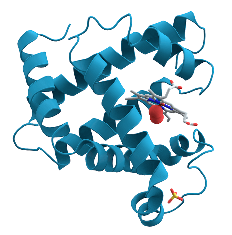
This effect plays a role on the conformation of proteins in aqueous media. Depending on the environmental conditions, a protein will fold and unfold, hiding or revealing its hydrophobic cores and its binding sites, thus impacting its activity.

What is true for water, is also true for other solvents. In general, the solvent is responsible for ‘hydrating’ the solute molecule and it is a major factor in solubility measurement. This is why the solubility of a drug in pure water is different from the solubility in water mixed with DMSO, another solvent.

The solute molecule can also influence the liquid around it. But before that, we need to understand how the structure of the solvent works.

The structure of a liquid – how the solvent affects itself

A pure solvent is a liquid made of identical molecules, that move next to each other and are linked by a variety of forces. Different interactions (attractive or repulsive) are involved:

  • the strong covalent/chemical bonding force (short range, attractive)
  • the electrostatic interaction between charged molecules
  • the charge-dipole interaction between a charged molecule and one that is uncharged but polarized
  • the dipole-dipole interaction between two dipoles
  • the hydrogen-bond, that is a strong type of directional dipole-dipole interactions
  • the so-called Van-der-Walls forces that are weak and often called dispersion forces
  • the repulsive forces (short-range), that prevents molecules to collide and fuse between each other

What you should remember here is that the molecules in the liquid will repel or attract each other depending on these interactions, in a very dynamic and fast manner.

These interactions, especially the short-range ones, give a very unique structure/molecular ordering to each liquid. For instance, strong hydrogen-bonding molecules can create dimers (e.g., fatty acids), linear 1D chains or rings (e.g., alcohols, hydrofluoric acid), 2D layered structures (e.g., formamide), or 3D structures (water).

And the liquid properties are determined by this ordering. For instance, if a liquid has a strong hydrogen-bonding, it will have a higher melting or boiling point (it will melt from the solid phase, or boil into a gas, at higher temperature). This is especially crucial in the case of water: its freezing/melting and boiling points make it perfect to be the ‘liquid of life’ on Earth.

The solvent is affected by the solute

The solvent structure rests on a subtle balance of the interactions mentioned above. But what happens when one introduces a solute (a different molecule) in it? The solute will add new interactions that will change the structure of the liquid and its properties.

A first example is when you add a charged solute to a solvent, such as salt to water: it does not freeze as easily as pure water. Sea water is very rarely frozen, will it is more common for the surface of a lake. This is because the addition of a salt that dissolves in water will introduce charged ions in the liquid. Then the charge-dipole interaction between the ion and the water dipoles will reorient the water molecules around it on a fairly long distance. This reorientation competes with the usual process of freezing (reorienting the water molecules to form an ice crystal) that happens usually at 0°C.

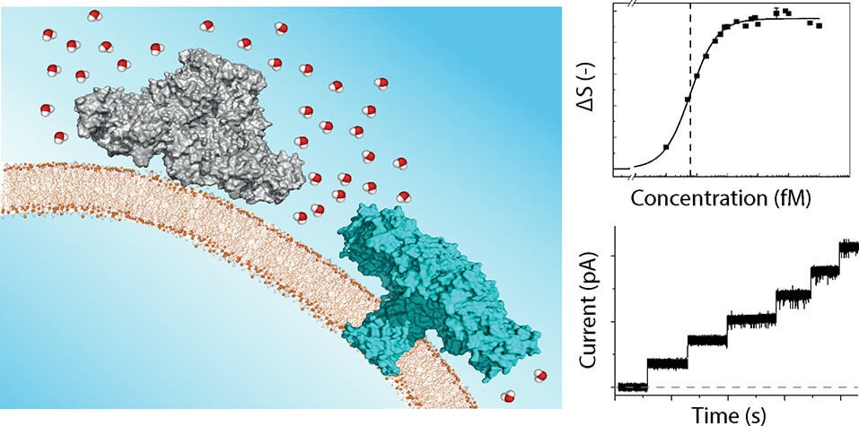
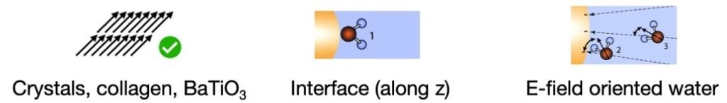
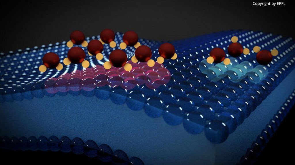
Confinement is another case of influence of the solute on the solvent. The insertion of a big molecule or an interface (oil droplet, lipid membrane, etc) that is insoluble in the liquid creates a boundary, a new frontier that blocks and alter the dynamics and structure of the liquid in its immediate vicinity. Confinement can be described as one-dimensional (next to a planar surface for instance), two-dimensional (water inside a pore or a nanotube), or three-dimensional (e.g., within a vesicle or a cell). Because of it, the solvent molecules experience less degrees of freedom to move, reorient, and interact with each other (it can make less hydrogen-bonds). Researchers have observed a broad range of effects caused by the solute such as slower relaxation times, changes in thermodynamics, freezing transitions, etc, compared to the bulk solvent far away from the solute.

Scientists found that these perturbations of the balance of interactions manifest on different time- and length-scales. They are stronger in the vicinity of the solute, and decreasing when going away from it, extending up to hundreds of nanometer in some cases.

However, investigating the solvent behavior at these scales is challenging, and this reflects in the plethoric lexical field used to interpret the influence of the solute. Here are some examples for the case of water:

  • It is often stated that water gets an ‘icelike’ structure next to big solutes, or properties similar to cooled or supercooled water. While not completely wrong, this is misleading as these changed properties come not from the solid state of water (i.e. ice) but from the solute presence.
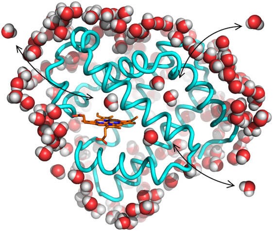
  • In a similar spirit, some coined the term of ‘biological water’ for water molecules next to proteins. While water has indeed an extreme importance in biology, this tends to hide the fact that the solute molecule itself carries the biological function.
  • Finally, the motion coupling of water and biological solutes has been described as water ‘slaving’ the solute motions. This is maybe a more accurate way of describing the mutual influences between the solute and the solvent molecules.

Studying these mutual influences between solvent and solutes is a challenge of extreme difficulty. Oryl has developed a groundbreaking technique to look at the reorientation if the solvent around a solute.

More information

The Solvent Redistribution method

What is the Solvent Redistribution (SR) method?

The solvent redistribution (SR) method is based on observing the redistribution of the solvent in response to an external stimulus such as the addition of solutes, changes in pH, temperature or pressure. The solvent is not simply a background but an active medium that responds to the smallest amounts of external stimulus.

Solvent Redistribution method as applied to solubility and aggregation

Solubility is about the solute dissolving in the solvent. Its not only about the solute but also about the solvent molecules around the solute! The SR method utilizes how the solvent redistributes around the solute molecules (it can be solid, liquid or gas) to obtain information about the aggregation state of the solute clusters. Here we show the redistribution of the solvent at different stages of aggregation:

Following the different stages of aggregation using the Solvent Redistribution method. With increasing concentration of solute in solution, solute monomers transition to stable aggregates. In-between fully dissolved monomers and stable aggregates, there is a concentration range where different types of solute structures (dimers, trimers, etc.) co-exist. Correspondingly, the solvent molecules around these dynamic structures redistribute and fluctuate. The technology behind the Solvent Redistribution method is called second harmonic scattering that directly measures the solvent molecules around the solute structures. At the onset of aggregation (the transition from monomers to dimers, trimers), the number of solvent molecules around the solute structures increases. This increase in interfacial solvent molecules lead to a steep increase in the second harmonic scattering intensity, which is used as a metric to measure the solubility limit.

How does the SR method change the landscape of solubility measurements?

The SR method is introducing a fundamental change on how solubility and aggregation is measured. While typical methods focus on observing the solute, the SR method shifts its focus on the solvent itself, which is an active medium. Small additions of solute is felt as a whole by the solvent molecules, making it sensitive to small additions (nanomolar concentrations) of solute. The solvent redistribution method is not limited to solubility measurements. It is also applicable to measurements of aggregation, crystallization and stability of substances. It has a wide application coverage, from different types of samples to different types of solvents. The only condition is that the solvent must be dipolar (e.g., water or any aqueous-based biologically relevant media, DMSO, methanol, ethanol and so forth). The solutes can be small molecules, fragments, proteins and macromolecules.

The SR method, as a light scattering technique is rapid and sensitive and requires minimum amount of compounds (read our Application Note here). It uses the solvent that is native and fundamental to the chemistry of solubility and aggregation. The SR method does not require the use of filters, filter-plates, vials, columns, and minimizes the use of chemicals and consumables, a sustainable and economical method for solubility and aggregation measurements.

More information

Spatiotemporal Imaging of Water in Operating Voltage-Gated Ion Channels Reveals the Slow Motion of Interfacial Ions

Ion channels are responsible for numerous physiological functions ranging from transport to chemical and electrical signaling. See the full paper here

3D imaging of surface chemistry in confinement

Check out the full paper here

High throughput second harmonic imaging for label-free biological applications

Second harmonic generation (SHG) is inherently sensitive to the absence of spatial centrosymmetry, which can render it intrinsically sensitive to interfacial processes, chemical changes and electrochemical responses. See full paper here

Chemistry of Lipid Membranes from Models to Living Systems

Lipid membranes provide diverse and essential functions in our cells relating to transport, energy harvesting and signaling. See full paper here.

A single ion impacts a million water molecules

Check out the full paper here.

Using water molecules to read electrical activity in lipid membranes

Check out the full paper here.